Analyzing and Comparing Deep Learning Models

This article data science blogthon.

Deep learning is a subset of machine learning. Deep learning is established on artificial neural networks to mimic the human brain. Deep learning adds a few hidden layers to gather the most detailed information and learn data for predictive modeling.

As with deep learning, the lack of processing power didn’t bother everyone. With today’s exponential growth in processing power, deep learning implementations are a hot topic.

Deep belief networks, deep neural networks, and recurrent neural networks are some of the deep learning models. In this article, we compare three models consisting of CNN (Convolution Neural Network), DNN (Deep Neural Network), and LSTM (Long Short-Term Memory).

The MNIST dataset is the best way to start working and practicing image-based datasets, so the application of this algorithm is to go one step further in medical images to classify and predict signs. The working implementations below demonstrate the broad ease of use for working with, implementing, and practicing the full spectrum of image datasets.

Check dataset

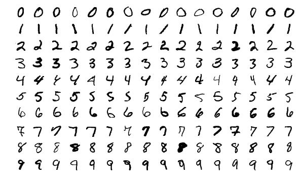
Here we use the MNIST dataset of handwritten digits ranging from 0 to 9. This dataset is split into two parts, a training set and a test set for prediction. The MNIST dataset is imported into a Jupyter notebook using the sklearn library.

Source: https://en.wikipedia.org/wiki/MNIST_database

Implementation

Implementation is done in Jupyter Note. The whole implementation is my Kaggle. Here’s the link:

Notebook link: https://www.kaggle.com/code/shibumohapatra/cnn-dnn-lstm-comparison

Library prerequisites

First, import the library of algorithms. Here are the libraries and their usage:

1. Bumpy: To manipulate arrays
2. panda: information processing
3. TensorFlow: Model Tracking for Prediction
4. Matplotlib: plot the graph
5. Keras: TensorFlow APIs
6. Tensorflow.keras.models: Build a machine learning model. Import a Sequential (a stack of layers with only one input tensor and one output tensor).
7. Sklearn model: Split the data into training and test sets
   
8. Tensorflow.keras.layers: Import various layers to implement deep learning. A description of the layers is given below –

• • Dense: Create a feedforward neural network. In other words, all inputs and all outputs are interdependent.
  • Flattening: Serialization of multidimensional tensors.
  • drop out: to prevent overfitting.
  • conv2D: A 2D convolution layer for maintaining relationships between pixels in image data.
  • MaxPooling2D: reduce the space s

from tensorflow.keras.models import Sequential
from tensorflow.keras.layers import Conv2D, MaxPooling2D, Dense, Flatten, Dropout, LSTM
from tensorflow.keras.utils import normalize
from sklearn.model_selection import train_test_split

data exploration

Here we load the MNIST data and split it into four sets: train_x, train_y, test_x, and test_y sets. After that, we normalize the train_x and test_x sets and output their respective data shapes. Next, view the dataset to make sure your exploration is correct. I have implemented a for loop to plot the 4 images of the dataset.

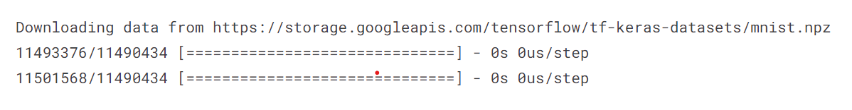
from keras.datasets import mnist
(train_x, train_y), (test_x, test_y) = mnist.load_data()

train_x = train_x.astype('float32')
test_x = test_x.astype('float32')
train_x /= 255
test_x /= 255
train_x = train_x.reshape(train_x.shape[0], 28, 28, 1)
test_x = test_x.reshape(test_x.shape)

# train set
print("The shape of train_x set is:",train_x.shape)
print("The shape of train_y set is:",train_y.shape)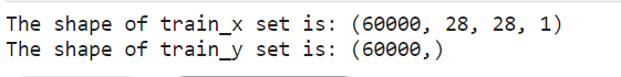

Training to set the shape of the MNIST dataset

# test set
print("The shape of test_x set is:",test_x.shape)
print("The shape of test_y set is:",test_y.shape)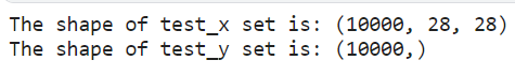

The test set the shape of the MNIST dataset

for i in range(1):  
  plt.subplot(330 + 1 + i)
  plt.imshow(train_x[i].reshape(28,28), cmap=plt.get_cmap('gray'))
  plt.axis('off')
  plt.show()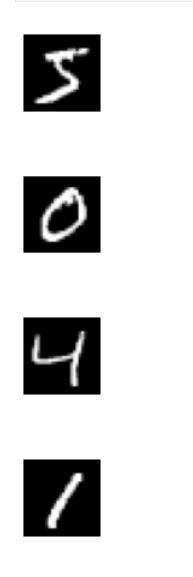

First 4 handwritten digits from the MNIST dataset

data load

After implementing more data exploration, we need to load the MNIST dataset and split it into four parts: x_train, y_train, x_test, y_test. Next, normalize the training and test sets to maintain consistency. Then return the normalized training and test sets.

Load DNN and RNN (LSTM) Data

Load the DNN and RNN (LSTM) data with the def load_data_NN() function, load the dataset, and perform normalization.

def load_data_NN():
  # load mnist dataset
  mnist = tf.keras.datasets.mnist  # 28 x 28 images of 0-9
  (x_train, y_train), (x_test, y_test) = mnist.load_data()
  # normalize data
  x_train = normalize(x_train, axis = 1)
  x_test = normalize(x_test, axis = 1)
  return x_train, y_train, x_test, y_test

Loading

For CNN, define the def load_data_CNN() function to load split the dataset and reshape the training and test sets.

CNNs involve convolutional layers, max pooling, flattening, and dense layers, which require reshaping. Here, the training and test sets are reshaped to 28 x 28 x 1 (28 rows, 28 columns, 1 color channel).

def load_data_CNN():
  # load mnist dataset
  mnist1 = tf.keras.datasets.mnist  # 28 x 28 images of 0-9
  (x_train, y_train), (x_test, y_test) = mnist1.load_data()
  # reshape data
  x_train = x_train.reshape(x_train.shape[0], 28, 28, 1)
  x_test = x_test.reshape(x_test.shape[0], 28, 28, 1)
  # convert from integers to floats
  x_train = x_train.astype('float32')
  x_test = x_test.astype('float32')
  # normalize data
  x_train = normalize(x_train, axis = 1)
  x_test = normalize(x_test, axis = 1)
  return x_train, y_train, x_test, y_test

Definition of Model 1 – DNN (Deep Neural Network)

A DNN is based on an artificial neural network and has several hidden layers between the input and output layers. DNNs are well suited for modeling complex nonlinear relationships. The main purpose here is to give the input, implement progressive computation in the input layer, and display or present the output to solve the problem. A deep neural network (DNN) is considered a feed forward network. In feed-forward networks, data does not flow backwards from the input layer to the output layer, and the links between layers are unidirectional. This means that the process will proceed without touching the node again.

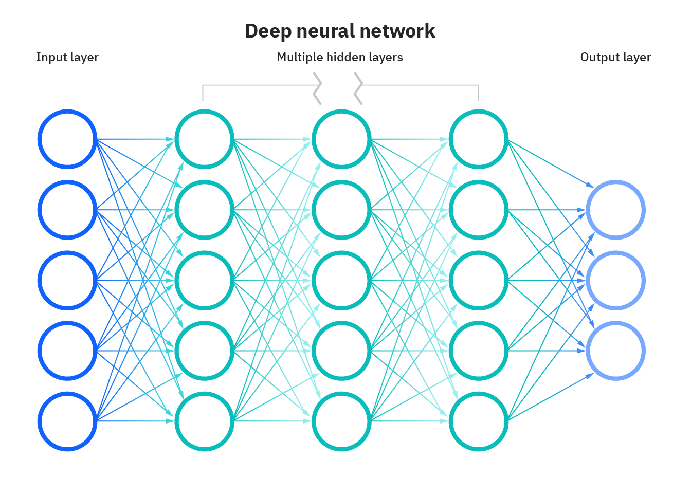
Source: https://www.ibm.com/cloud/learn/neural-networks

For DNN, sequential, flattened, and three dense layers are implemented. The first two dense layers have 128 nodes and a ReLU activation function. In the third dense layer, we defined 10 nodes and a softmax activation function.

def DNN():
  model_dnn = Sequential()
  model_dnn.add(Flatten())  # input layer
  model_dnn.add(Dense(128, activation = 'relu'))
  model_dnn.add(Dense(128, activation = 'relu'))
  model_dnn.add(Dense(10, activation = 'softmax'))
  model_dnn.compile(optimizer= "adam", 
                  loss= "sparse_categorical_crossentropy", metrics=["accuracy"])
  return model_dnn

I compiled a DNN model to use the Adam optimizer and a sparse categorical cross-entropy (multiclass classification model with integer values ​​assigned to the output labels) loss function. The accuracy of the model determines the metric.

Definition of Model 2 – RNN (LSTM)

RNN is short for Recurrent Neural Network and is adapted to work with time-series or sequence data.

Here we implement an LSTM that can be viewed as an RNN. A Long Short-Term Memory (LSTM) is a special kind of RNN that can learn long-term dependencies. This helps the RNN remember what happened in the past to make reasonable next estimates.

Using LSTMs solves the problem of long-term dependencies in RNNs. RNNs could not store words in long-term dependencies, but based on recent information, RNNs could predict them more accurately. However, the RNN does not perform optimally as the gap length increases. The solution is her LSTM, which retains information for a longer period of time, reducing data loss. Applications of LSTM are used for classification and forecasting of time series data.

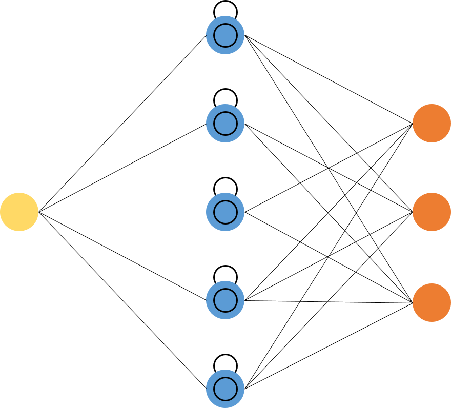
Source: https://i.stack.imgur.com/h8HEm.png

DNN (LSTM) – LSTM layers, sequential, dropout layers (0.2 drops out 20% of nodes to prevent overfitting), and dense layers. The layer above has a ReLU and a softmax activation function. I compiled an LSTM model and used the Adam optimizer and a loss function (sparse categorical cross-entropy). The accuracy of the model determines the metric.

def RNN(input_shape):
  model_rnn = Sequential()
  model_rnn.add(LSTM(128, input_shape=input_shape, activation = 'relu', return_sequences=True))
  model_rnn.add(Dropout(0.2))
  model_rnn.add(LSTM(128, input_shape=input_shape, activation = 'relu'))
  model_rnn.add(Dropout(0.2))
  model_rnn.add(Dense(32, activation = 'relu'))
  model_rnn.add(Dropout(0.2))
  model_rnn.add(Dense(10, activation = 'softmax'))
  model_rnn.compile(optimizer= "adam", 
                  loss= "sparse_categorical_crossentropy", metrics=["accuracy"])
  return model_rnn

Definition of Model 3 – CNN (Convolutional Neural Network)

CNN is a category of artificial neural networks. CNNs are widely used for object recognition and classification in deep learning. Using CNN, deep learning detects objects in images. Convolutional neural networks (CNNs, or ConvNets) are a class of deep neural networks most commonly applied to the analysis of visual images. Applications of CNN are video understanding, speech recognition, and NLP understanding. A CNN has an input layer, an output layer, one or more hidden layers, and a large number of parameters, allowing CNNs to learn complex patterns and objects.

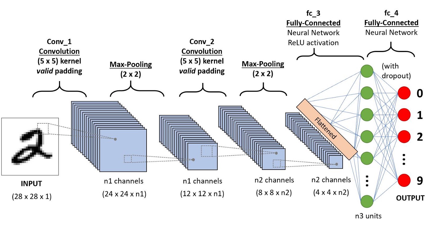
Source: https://miro.medium.com/max/1400/1*uAeANQIOQPqWZnnuH-VEyw.jpeg

For CNN, follow Sequential and add Conv2D layer, MaxPooling2D layer and Dense layer. The ReLU and softmax activation functions are similar to the model above. I compiled an LSTM model and used the Adam optimizer and a loss function (sparse categorical cross-entropy). The accuracy of the model determines the metric.

def CNN(input_shape):
  model_cnn = Sequential()
  model_cnn.add(Conv2D(32, (3,3),  input_shape = input_shape))
  model_cnn.add(MaxPooling2D(pool_size=(2,2)))
  model_cnn.add(Flatten())  # converts 3D feature maps to 3D feature vectors
  model_cnn.add(Dense(100, activation='relu'))
  model_cnn.add(Dense(10, activation='softmax'))
  model_cnn.compile(loss="sparse_categorical_crossentropy",
                 optimizer="adam", metrics=["accuracy"])
  return model_cnn

prediction phase

The implementation below is useful for predicting and verifying prediction output for specific or individual indices of an image dataset.

Now you can use the model you built to train and test your dataset.

def sample_prediction(index):
  plt.imshow(x_test[index].reshape(28, 28),cmap='Greys')
  pred = model.predict(x_test[index].reshape(1, 28, 28, 1))
  print(np.argmax(pred))

DNN model prediction

For the DNN to make the first prediction, load the load_data_NN() function, load and fit the model in 5 epochs. After evaluating and testing that model, the accuracy is obtained and finally we define a sample image to ensure that the model is predicting the image with maximum accuracy.

if __name__ == "__main__":
  # load data
  x_train, y_train, x_test, y_test = load_data_NN()
  # load the model
  model = DNN()
  print("nnModel Trainingn")
  model.fit(x_train, y_train, epochs = 5)
  print("nnModel Evaluationn")
  model.evaluate(x_test, y_test)
  score1 = model.evaluate(x_test, y_test, verbose=1)
  print('n''DNN Model Test accuracy:', score1[1])
  print("nnSample Prediction")
  sample_prediction(20)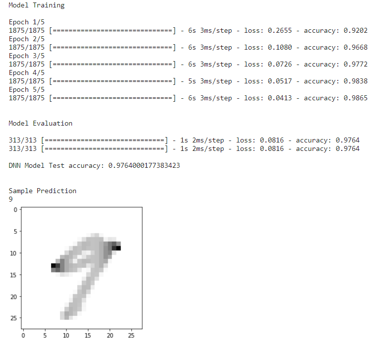

DNN model prediction

RNN (LSTM) model prediction

The RNN (LSTM) and DNN approaches are the same as the model.

if __name__ == "__main__":
  # load data
  x_train, y_train, x_test, y_test = load_data_NN()
  # load model
  model = RNN(x_train.shape[1:])
  print("nnModel Trainingn")
  model.fit(x_train, y_train, epochs = 5)
  print("nnModel Evaluationn")
  model.evaluate(x_test, y_test)
  score2 = model.evaluate(x_test, y_test, verbose=1)
  print('n''RNN (LSTM) Model Test accuracy:', score2[1])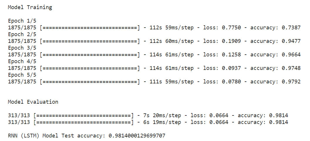

RNN (LSTM) model prediction

CNN Model Prediction

For CNN, load the load_data_CNN() function. The CNN function is different from the other two because it has convolutional layers, congestion, flattening, etc. In addition to the training and test sets, they also differ in size. This bespoke feature is beneficial to CNN.

if __name__ == "__main__":
  # load data
  x_train, y_train, x_test, y_test = load_data_CNN()
  # load model
  input_shape = (28,28,1)
  model = CNN(input_shape)
  print("nnModel Trainingn")
  model.fit(x_train, y_train, epochs = 5)
  print("nnModel Evaluationn")
  model.evaluate(x_test, y_test)
  score3 = model.evaluate(x_test, y_test, verbose=1)
  print('n''CNN Model Test accuracy:', score3[1])
  print("nnSample Prediction")
  sample_prediction(20)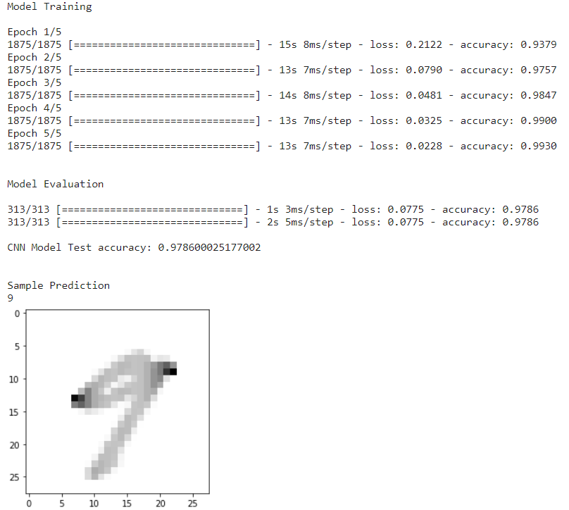

CNN Model Prediction

After loading the CNN function, it’s time to fit the model in 5 epochs. After evaluation and testing of that model, we have the accuracy and we have a sample input image to predict the image.

Comparison of model accuracy

After implementing the three models and getting their scores, we need to compare them to arrive at a final statement. The code below shows a tabular format showing the accuracy of the model from best to worst.

The code says to call the model and its accuracy in array form, sort in descending order, and display the output in tabular form.

results=pd.DataFrame({'Model':['DNN','RNN (LSTM)','CNN'],
                     'Accuracy Score':[score1[1],score2[1],score3[1]]})
result_df=results.sort_values(by='Accuracy Score', ascending=False)
result_df=result_df.set_index('Model')
result_df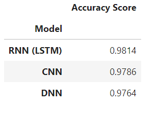

Model accuracy table

The table generated above shows that RNN (LSTM) leads the prediction with maximum accuracy score, while CNN has 2^nd location, which gives the DNN the lowest accuracy score.

Conclusion

To summarize the entire run:

1. I have imported the library.explored and loaded Create a dataset by plotting some images.
2. We then defined two tuned creation functions for DNN, RNN (LSTM) and CNN.
3. I implemented the algorithm in each deep learning model.
4. After that, we started with the prediction phase for all deep learning models.
5. Finally, we created a comparison table to see which deep learning models are good at predicting the MNIST dataset.

Therefore, the RNN (LSTM) model is the overall winner with a score of 98.54%. CNN model is 2^nd 98.08%, DNN model ranked third^rd 97.21% of places. Here are the main points of the final comparison table:

• Due to the short implementation time, fewer parameters are required to train the CNN model and the model performance is preserved.
• The faster the execution, the more parameters the DNN model needs to train, but the model’s performance suffers with less accuracy.
• The LSTM with the slowest execution time performed better than the other two. This improves LSTM performance.
• Therefore, with the above implementation, we can conclude that the LSTM model is suitable for deep learning to process MNIST and other image datasets.

I hope this article helps you understand how to choose the right deep learning model. Thank you.

Media shown in this article are not owned by Analytics Vidhya and are used at the author’s discretion.

Related